SharpPlot Tutorials > Chart Samples > Contour plots for XYZ interpolation

Contour plots for XYZ interpolation

Contour plots offer a 2-dimensional alternative to CloudCharts when it is necessary to visualize ‘height’ data in addition to x and y values. The data may be geographic (rainfall totals from a number of weather stations) or simply a model of 3 variables (house prices as a function of the age of the property and its floor area).

Depending on the type of data, SharpPlot can fit a variety of models to generate the contours for the height dimension. These four examples show how very similar numbers can create very different maps depending on the chosen approach. The key properties are the order of fit (which creates an underlying model) and flexibility (which determines how far the computed surface can deviate from the model).

Note that the ContourPlot is just an extension of the simple ScatterPlot, and shares many of its style settings.

A Simple 2-variable Regression Surface

This example fits the same Quadratic surface as the third CloudChart tutorial. You can see that several of the points fall on the ‘wrong’ side of the line, which is very reasonable for a noisy dataset where the Z-values may be subject to a large random error.

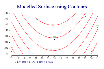
sp.Heading = "Modelled Surface using Contours";

zdata = new int[] {12,65,77,117,9,112};
xdata = new int[] {17,31,29,21,30,24};
ydata = new int[] {190,270,310,300,190,230};

sp.SetOrderOfFit(2,1);
sp.Flexibility = 0;
sp.EquationFormat = "z = C0 + C1x + C2x² + C3y";

sp.ContourPlotStyle = ContourPlotStyles.ValueTags|ContourPlotStyles.ExplodeAxes|
         ContourPlotStyles.Curves;
sp.SetMarkers(Marker.Bullet);

sp.DrawContourPlot(xdata,ydata,zdata);
sp.SetKeyText(sp.Equation);

The Cloudchart is probably a better tool for an initial visualisation, but the Contourplot is much more suitable if you want to answer questions like “what is the best estimate for z, given x and y” as you can easily read off he numbers.

An Approximate Trend Surface

The remaining examples all use the same set of data-points as the final example in the Cloudchart tutorial. The same data-set can produce very different ‘landscapes’ depending on the model chosen.

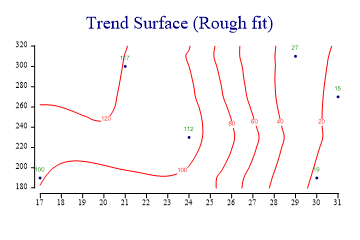
zdata = new int[] {100,15,27,117,19,112};
xdata = new int[] {17,31,29,21,30,24};
ydata = new int[] {190,270,310,300,190,230};

sp.Heading = "Trend Surface (Rough fit)";

sp.ContourPlotStyle = ContourPlotStyles.ValueTags|ContourPlotStyles.ExplodeAxes|
         ContourPlotStyles.Curves;
sp.SetMarkers(Marker.Bullet);

sp.Flexibility = 5;
sp.MeshDensity = 2;

sp.DrawContourPlot(xdata,ydata,zdata);

The first surface shows the effect of setting the flexibility quite low. Each computed point on the xy grid then ‘sees’ many of the nearby points and the effect is create a quite smooth (but strongly averaged) surface. This would be a suitable model if the data were known to be noisy, and a rough feel for the shape of the surface was all that was required.

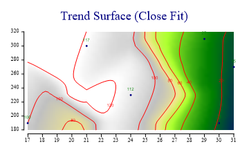
Fitting an Accurate set of Spot-heights

If the z-values really represent accurately measured values (spot heights in a landscape) then the map should be forced to fit itself around them.

zdata = new int[] {100,15,27,117,19,112};
xdata = new int[] {17,31,29,21,30,24};
ydata = new int[] {190,270,310,300,190,230};

sp.Heading = "Trend Surface (Close Fit)";
sp.SetAltitudeColors(new Color[]{Color.Navy,Color.Green,Color.GreenYellow,
         Color.Khaki,Color.Silver,Color.White});
sp.ContourPlotStyle = ContourPlotStyles.ValueTags|ContourPlotStyles.ExplodeAxes|
         ContourPlotStyles.AltitudeShading;
sp.SetMarkers(Marker.Bullet);

sp.Flexibility = 8;
sp.MeshDensity = 5;

sp.DrawContourPlot(xdata,ydata,zdata);

This example increases the mesh-density (to compute the contours at many more points) and sets the flexibility high enough to force the contours to behave correctly with respect to the points nearby. Whether this map is any better than any other is (of course) arguable. It is an interesting exercise to take a set of points like this and attempt to make the map by hand. Altitude shading has been used with ‘realistic’ colouring to give the effect of an aerial view of a landscape.

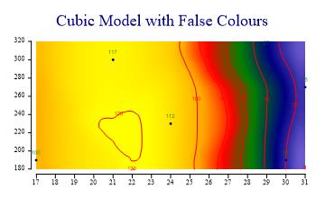
Fitting a Flexible Cubic Model

The final example generates the most ‘satisfying’ map, from a purely visual point of view. This allows SharpPlot to fit a cubic regression surface in the x-direction, then apply a little flexibility to this to finalise the shape of the surface. No underlying model is assumed in the y-direction.

zdata = new int[] {100,15,27,117,19,112};
xdata = new int[] {17,31,29,21,30,24};
ydata = new int[] {190,270,310,300,190,230};

sp.Heading = "Cubic Model with False Colours";
sp.SetAltitudeColors(new Color[]{Color.SlateBlue,Color.Navy,Color.Green,Color.Red,
         Color.Orange,Color.Yellow});

sp.ContourPlotStyle = (ContourPlotStyles.ValueTags|ContourPlotStyles.ExplodeAxes|
         ContourPlotStyles.AltitudeShading|ContourPlotStyles.Curves);
sp.SetMarkers(Marker.Bullet);

sp.SetOrderOfFit(3,0);
sp.Flexibility = 8;
sp.MeshDensity = 3;

sp.DrawContourPlot(xdata,ydata,zdata);

This combination of modelfit and flexibility is a good approach when you know that the z-value is composed of several effects, some of which are expected to obey a known model, but some of which are effectively ‘random’ values. Altitude shading can be used with an array of suitable color values to help bring out the shape of the final surface.

Summary

Contour plots can be an excellent way to display 3-dimensional data on a 2-dimensional chart, but creating the ‘best’ surface for any given dataset will require some prior knowledge of the underlying model, and a certain amount of experimentation.

Send comments on this topic
© Dyalog Ltd 2021